The key usage of AmyPET Centiloid (CL) analysis.
This is the multi-page printable view of this section. Click here to print.
Tutorials
Multiple examples of AmyPET usage
1 - Amyloid PET Centiloid Pipeline
Understanding the output of the Centiloid (CL) processing pipeline, including QC.
Below is presented a pipeline for CL analysis of static amyloid brain PET scan using [18F] florbetaben radiotracer.
The scan consists of four 5-minutes frames which are first aligned and then processed for CL.
First, import all necessary Python packages
from pathlib import Path
import numpy as np
from matplotlib import pyplot as plt
from niftypet import nimpa
import spm12
import amypet
from amypet import backend_centiloid as centiloid
from amypet import params as Cnt

import logging
logging.basicConfig(level=logging.INFO)
Set up the input and output
# > ignore derived DICOM files
ignore_derived = False

# > uptake ratio (UR) window def (unfortunately, aka SUVr)
ur_win_def = [5400,6600]

# > type of amyloid radiopharmaceutical, here [18F]florbetaben
tracer = 'fbb'

# > input PET folder
input_fldr = Path('/home/pawel/data/PNHS/FBB1_STAT')

# > output path
outpath = input_fldr.parent/('amypet_output_'+input_fldr.name)
Please note that not infrequently DICOM fields have wrong tracer information recorded, e.g., FDG instead of an amyloid tracer name. Hence it is always safer to define this prior to the analysis as it is done above.
It is also important to note that for a proper functioning of this pipeline there are DICOM fields which cannot be missing about the PET acquisition - see below for details.
Explore, identify DICOM files and convert to NIfTI
Please note, that in order to obtain the relevant information about PET acquisition, key DICOM fields have to be present. Among others (such as image orientation and size), these are:
- study time and date
- series time
- acquisition time
- frame duration time
- time of tracer administration (start)
- PET tracer name (not always accurate or present; can be overwritten by specifying it upfront when running AmyPET).
#------------------------------
# > structural/T1w image
ft1w = amypet.get_t1(input_fldr, Cnt)

if ft1w is None:
    raise ValueError('Could not find the necessary T1w DICOM or NIfTI images')
#------------------------------

#------------------------------
# > processed the PET input data and classify it (e.g., automatically identify UR frames)
indat = amypet.explore_indicom(
    input_fldr,
    Cnt,
    tracer=tracer,
    find_ur=True,
    ur_win_def=ur_win_def,
    outpath=outpath/'DICOMs')

# > convert to NIfTIs
niidat = amypet.convert2nii(indat, use_stored=True)
#------------------------------
Align the dynamic/static frames
This does not have to be executed if only one PET frame is available. The alignment can be done with SPM or DIPY registration tools.
aligned = amypet.align(
    niidat,
    Cnt,
    reg_tool='spm',
    ur_fwhm=4.5,
    use_stored=True)
CL quantification
# > optional CSV file output for CL results
fcsv = input_fldr.parent/(input_fldr.name+'_AmyPET_CL.csv')

out_cl = centiloid.run(
    aligned['ur']['fur'],
    ft1w,
    Cnt,
    stage='f',
    voxsz=1,
    bias_corr=True,
    tracer=tracer,
    outpath=outpath/'CL1',
    use_stored=True,
    #fcsv=fcsv
    )
Exploring the output
The output dictionary out_cl contains the following outputs:
out_cl['fmri']: file path to the original input T1w MRI image.
out_cl['n4']: output of the bias field correction for the T1w MRI image.
out_cl['mric']: output of the centre-of-mass correction for the MRI image, including output file path as well as relative and absolute translation parameters.
out_cl['petc']: output of the centre-of-mass correction for PET image, including output file path as well as relative and absolute translation parameters.
Please note that all the output for centre-of-mass corrections are stored in subfolder centre-of-mass inside the output folder out_cl['opth'].
out_cl['fpet']: the path to the CL input PET after alignment which includes centre of mass adjustment to facilitate more robust SPM registration/alignment.
out_cl['reg1']: output of the affine MRI registration to the MNI space template; output includes the path to the registered MRI image, path to the affine transformation file, and the affine transformation array itself.
out_cl['reg2']: output of the affine PET registration to the above registered MRI image; output includes the path to the registered PET image, path to the affine transformation file, and the affine transformation array itself.
Please note that all that all the affine registration output is stored in subfolder registration in the output folder out_cl['opth'].
out_cl['norm']: output of all the SPM normalisation/segmentation, including paths to the parameters, inverse and forward transfromations as well as the grey (c1) and white (c2) matter segmentation probability masks.
out_cl['fnorm']: is the list of all the paths of spatially normalised files, including the MRI, PET and grey/white matter segmentation probability masks.
out_cl['avgvoi']: is the output dicionary of average volume of interest (VOI) values for the Centiloid masks of the cerebellum grey matter (cg), the whole cerebellum (wc), the whole cerebellum + brain stem (wcb), the pons (pns) and the cortex (ctx).
out_cl['ur']: are the uptake ratio values (unfortunately also known as SUVr) for the cerebellum grey matter (cg), the whole cerebellum (wc), the whole cerebellum + brain stem (wcb), the pons (pns) reference regions.
out_cl['ur_pib_calc']: these are the [C11]PiB converted values to the above.
out_cl['ur_pib_calc_transf']: are the saved linear transformation parameters.
Main output:
out_cl['cl']: the Centiloid (CL) values for each reference region, that is the cerebellum grey matter (cg), the whole cerebellum (wc), the whole cerebellum + brain stem (wcb), the pons (pns).
out_cl['fcsv']: the path to the CSV file with all the outputs.
out_cl['fqc']: the file path to the QC image showing all the sampling masks superimposed on the PET image in transaxial and sagittal views together with printed all the CL and UR values.
Image Output:
The key image output in NIfTI format for the CL converted images suing all the available reference regions (the cerebellum grey matter, the whole cerebellum, the whole cerebellum + brain stem , the pons) as well as the corresponding uptake ratio (UR) images (aka SUVr) are contained in the results subfolder folder.
The QC image for the Centiloid pipeline can be viewed as follows:
from PIL import Image

fig,axs = plt.subplots(1,1, figsize=(16, 12))

# > show the QC image in PNG format for the the Centiloid pipeline
axs.imshow( np.asarray(Image.open(out_cl['fqc'])) )
axs.axes.get_xaxis().set_ticks([])
axs.axes.get_yaxis().set_ticks([])

Quality Control Checks
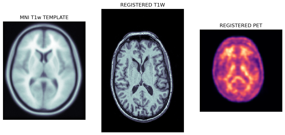
Viewing affine registered MRI and PET images
The first output of the CL pipeline are the registrations of T1w MRI image to the MNI template followed by the registration of PET to the MNI registered MRI image.
tmpl = nimpa.getnii(spm12.spm_dir()+'/canonical/avg152T1.nii')
t1wa = nimpa.getnii(out_cl['reg1']['freg'])
peta = nimpa.getnii(out_cl['reg2']['freg'])

fig,axs = plt.subplots(1,3, figsize=(12, 8))

axs[0].matshow(tmpl[50,...], cmap='bone')
axs[1].matshow(t1wa[95,...], cmap='bone')
axs[2].matshow(peta[40,...], cmap='magma')

# > remove ticks
for i in range(3):
    axs[i].axes.get_xaxis().set_ticks([])
    axs[i].axes.get_yaxis().set_ticks([])

axs[0].set_title('MNI T1w TEMPLATE')
axs[1].set_title('REGISTERED T1W')
axs[2].set_title('REGISTERED PET')
The plots below show the MNI template with the registered MRI and PET images.
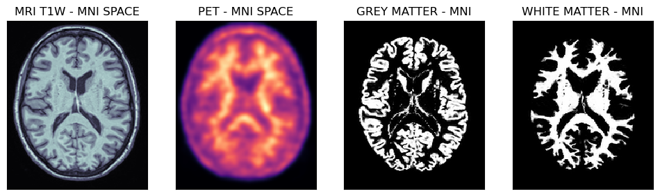
Viewing spatially normalised masks and MRI/PET images
Below are shown PET and MRI images spatially normalised to the MNI space. Note, that the voxel size is 1 mm isotropically, hence the probability masks for grey and white matter regions are well defined.
mrin = nimpa.getnii(out_cl['fnorm'][0])
petn = nimpa.getnii(out_cl['fnorm'][1])
gmn = nimpa.getnii(out_cl['fnorm'][2])
wmn = nimpa.getnii(out_cl['fnorm'][3])

fig,axs = plt.subplots(1,4, figsize=(12, 8))

axs[0].matshow(mrin[95,...], cmap='bone')
axs[1].matshow(petn[95,...], cmap='magma')
axs[2].matshow(gmn[95,...], cmap='gray')
axs[3].matshow(wmn[95,...], cmap='gray')

# > remove ticks
for i in range(4):
    axs[i].axes.get_xaxis().set_ticks([])
    axs[i].axes.get_yaxis().set_ticks([])

axs[0].set_title('MRI T1W - MNI SPACE')
axs[1].set_title('PET - MNI SPACE')
axs[2].set_title('GREY MATTER - MNI')
axs[3].set_title('WHITE MATTER - MNI')


fig,axs = plt.subplots(1,2, figsize=(10, 6))

axs[0].matshow(petn[95,...], cmap='magma')
axs[0].imshow(gmn[95,...], cmap='gray', alpha=0.3)
axs[1].matshow(petn[95,...], cmap='magma')
axs[1].imshow(wmn[95,...], cmap='gray', alpha=0.3)

# > remove ticks
for i in range(2):
    axs[i].axes.get_xaxis().set_ticks([])
    axs[i].axes.get_yaxis().set_ticks([])

axs[0].set_title('GM MASK IN PET')
axs[1].set_title('WM MASK IN PET')
Transaxial slices of the MRI and PET images in the MNI space together with the grey and white matter probability masks. Further below are shown the grey matter and white matter masks superimposed on the PET image.

2 - Atlas-Based MNI PET analysis
Use of the Centiloid (CL) output for the subsequent PET analysis in the MNI space with the available four brain atlases.
The analysis relies on the CL processing presented previously in the previous section Centiloid Pipeline.
The presented MNI space analysis of PET images may use either the MNI normalised PET images, or the output CL/UR images stored in the results subfolder in the output path stored in cl_out['opth'] - the output dictionary of the CL pipeline (see details here). For the MNI analysis a number of generally available atlases can be used as shown below.
Atlases Supported In AmyPET
The available atlases include:
- The Hammers atlas (you will be prompted to fill the online license).
- The DKT (Desikan-Killiany-Tourville) atlas.
- The Schaefer atlas.
- The AAL atlas.
# > get the available atlases in the MNI space as Python dicionaries
hmr = amypet.get_atlas(atlas='hammers')
dkt = amypet.get_atlas(atlas='dkt')
sch = amypet.get_atlas(atlas='schaefer')
aal = amypet.get_atlas(atlas='aal')
All the atlases come with the sub-dictionaries of available labels and names. For example, for the Hammers atlas, we can find the following dictionary items:
hmr.keys()
dict_keys(['fatlas', 'fatlas_full', 'flabels', 'voi_lobes', 'vois'])
with vois and voi_lobes representing the different labels for all the available volumes of interests (VOI) and the composite VOIs for the lobes of the brain. Please note that the Hammers atlas has the full version (including the white matter, WM) and the grey matter (GM) version.
Atlas resampling to the PET image size
Although the available atlases are already in the MNI space, they have a different image or voxel sizes. Hence they are interpolated with identity transformation to fully align them with the PET space which can have voxel size of either 1 or 2 mm isotropically.
# > Hammers atlas - the grey matter version
fhmr = spm12.resample_spm(
    out_cl['fnorm'][1],
    hmr['fatlas'],
    np.eye(4),
    intrp=0,
    fimout=Path(out_cl['fnorm'][1]).parent/('InPET_'+hmr['fatlas'].name),
    del_ref_uncmpr=True,
    del_flo_uncmpr=True,
    del_out_uncmpr=True)

# > Hammers atlas - full version with the WH
fhmrf = spm12.resample_spm(
    out_cl['fnorm'][1],
    hmr['fatlas_full'],
    np.eye(4),
    intrp=0,
    fimout=Path(out_cl['fnorm'][1]).parent/('InPET_'+hmr['fatlas_full'].name),
    del_ref_uncmpr=True,
    del_flo_uncmpr=True,
    del_out_uncmpr=True)

fdkt = spm12.resample_spm(
    out_cl['fnorm'][1],
    dkt['fatlas'],
    np.eye(4),
    intrp=0,
    fimout=Path(out_cl['fnorm'][1]).parent/('InPET_'+dkt['fatlas'].name),
    del_ref_uncmpr=True,
    del_flo_uncmpr=True,
    del_out_uncmpr=True)

fsch = spm12.resample_spm(
    out_cl['fnorm'][1],
    sch['fatlas'],
    np.eye(4),
    intrp=0,
    fimout=Path(out_cl['fnorm'][1]).parent/('InPET_'+sch['fatlas'].name),
    del_ref_uncmpr=True,
    del_flo_uncmpr=True,
    del_out_uncmpr=True)

faal = spm12.resample_spm(
    out_cl['fnorm'][1],
    aal['fatlas'],
    np.eye(4),
    intrp=0,
    fimout=Path(out_cl['fnorm'][1]).parent/('InPET_'+aal['fatlas'].name),
    del_ref_uncmpr=True,
    del_flo_uncmpr=True,
    del_out_uncmpr=True)
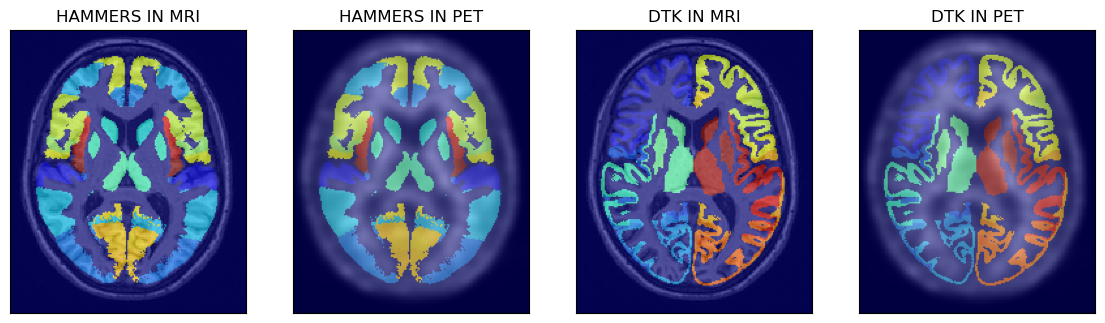
Exploring The Atlases
All the four available atlases are shown below after loading the atlases to Numpy arrays:
# > read the atlases to Numpy arrays
ihmr = nimpa.getnii(fhmr)
idtk = nimpa.getnii(fdkt)
isch = nimpa.getnii(fsch)
iaal = nimpa.getnii(faal)
# > show the first two atlases superimposed on MRI and PET images
fig,axs = plt.subplots(1,4, figsize=(14, 8))
axs[0].matshow(mrin[100,...], cmap='gray')
axs[0].imshow(ihmr[100,...], cmap='jet', alpha=0.6)
axs[1].matshow(petn[100,...], cmap='gray')
axs[1].imshow(ihmr[100,...], cmap='jet', alpha=0.5)
axs[2].matshow(mrin[100,...], cmap='gray')
axs[2].imshow(idtk[100,...], cmap='jet', alpha=0.6)
axs[3].matshow(petn[100,...], cmap='gray')
axs[3].imshow(idtk[100,...], cmap='jet', alpha=0.5)
# > remove ticks
for i in range(4):
axs[i].axes.get_xaxis().set_ticks([])
axs[i].axes.get_yaxis().set_ticks([])
# > image labels
axs[0].set_title('HAMMERS IN MRI')
axs[1].set_title('HAMMERS IN PET')
axs[2].set_title('DTK IN MRI')
axs[3].set_title('DTK IN PET')
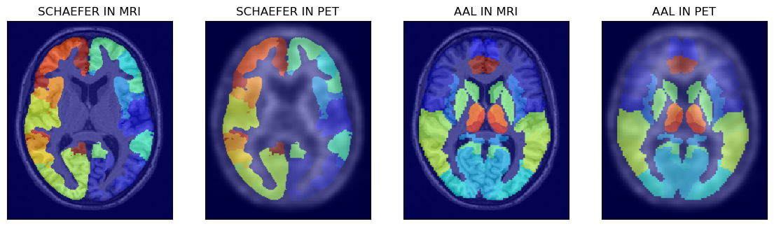
# > show the other two atlases superimposed on MRI and PET images
fig,axs = plt.subplots(1,4, figsize=(14, 8))
axs[0].matshow(mrin[100,...], cmap='gray')
axs[0].imshow(isch[100,...], cmap='jet', alpha=0.6)
axs[1].matshow(petn[100,...], cmap='gray')
axs[1].imshow(isch[100,...], cmap='jet', alpha=0.5)
axs[2].matshow(mrin[100,...], cmap='gray')
axs[2].imshow(iaal[100,...], cmap='jet', alpha=0.6)
axs[3].matshow(petn[100,...], cmap='gray')
axs[3].imshow(iaal[100,...], cmap='jet', alpha=0.5)
# > remove ticks
for i in range(4):
axs[i].axes.get_xaxis().set_ticks([])
axs[i].axes.get_yaxis().set_ticks([])
# > image labels
axs[0].set_title('SCHAEFER IN MRI')
axs[1].set_title('SCHAEFER IN PET')
axs[2].set_title('AAL IN MRI')
axs[3].set_title('AAL IN PET')
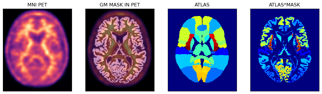
PET Image Analysis Using The Hammers Atlas And The GM Probability Mask
Below is an example of using the PET image in the MNI space with the corresponding GM probability mask (thus avoiding some partial volume problems during sampling) and the full Hammers atlas with segmentations for the GM and WM.
# > get the Numpy array representing the Hammers atlas image
ihmrf= nimpa.getnii(fhmrf)

# > the the Numpy array of the PET image in the MNI space
petmni = nimpa.getnii(out_cl['fnorm'][1])

# > get the corresponding GM probability mask Numpy array
gm_mni = nimpa.getnii(out_cl['fnorm'][2])

# > plot the images
fig,axs = plt.subplots(1,4, figsize=(14, 8))
axs[0].matshow(petmni[100,...], cmap='magma')
axs[1].matshow(petmni[100,...], cmap='magma')
axs[1].imshow(gm_mni[100,...], cmap='gray', alpha=0.5)
axs[2].matshow(ihmrf[100,...], cmap='jet')
axs[3].matshow(ihmrf[100,...]*gm_mni[100,...], cmap='jet')

# > remove ticks
for i in range(4):
    axs[i].axes.get_xaxis().set_ticks([])
    axs[i].axes.get_yaxis().set_ticks([])

axs[0].set_title('MNI PET')
axs[1].set_title('GM MASK IN PET')

axs[2].set_title('ATLAS')
axs[3].set_title('ATLAS*MASK');
Perform the extraction of average VOI values
For simplicity here we use the composite lobe VOIs:
vois = amypet.extract_vois(
    petmni,
    fhmrf, # uses full atals
    hmr['voi_lobes'],
    atlas_mask=gm_mni, # applies the GM mask on top of the full Hammers atals
    outpath=outpath/'MNI_masks', # path to the masks
    output_masks=True # output all the individual masks for each composite VOI
)
Average value for the cingulate gyrus
print('The average value in the cingulate gyrus is avg = {}. The number of voxles (also partial) is nvox = {}.'.format(vois['CG']['avg'], vois['CG']['vox_no']))
The average value in the cingulate gyrus is avg = 9066.670901759866. The number of voxels (also partial) is nvox = 26160.29958630912.
3 - Atals-Based Native PET analysis
Use of the Centiloid (CL) output for the subsequent native PET analysis.
The analysis relies on the CL processing presented previously here.
This native PET space analysis may use all the available MNI space atlases after transforming them to the PET space using the CL transformations.
Performing Analysis In The Native PET Space
The raw (unmodified) PET image is analysed without any transformation or filtering applied to the image. The output of this native analysis is stored in the native folder as shown below.
    # output for native PET analysis
    onat = outpath/'native'

    # > reference PET (explicitly identifying it from CL processing input)
    fpetin = out_cl['petc']['fim']

    # > get PET Numpy array
    pet = nimpa.getnii(fpetin)

    # > save the atlases and grey/white matter masks in the dictionary of native PET output
    natdct = amypet.atl2pet(hmr['fatlas_full'], out_cl, fpet=fpetin, outpath=onat)
The above natdct dictionary contains the file paths and images for the grey and white matter probabilistic masks as well as the atlas in the native PET space.
The native PET slices and registered masks and atlases are shown below using the Hammers atlas:
# > plot the images
fig,axs = plt.subplots(1,4, figsize=(14, 8))
axs[0].matshow(pet[40,...], cmap='magma')
axs[1].matshow(pet[40,...], cmap='magma')
axs[1].imshow(natdct['gmpet'][40,...], cmap='gray', alpha=0.5)
axs[2].matshow(natdct['atlpet'][40,...], cmap='jet')
axs[3].matshow(natdct['atlpet'][40,...]*natdct['gmpet'][40,...], cmap='jet')

# > remove ticks
for i in range(4):
    axs[i].axes.get_xaxis().set_ticks([])
    axs[i].axes.get_yaxis().set_ticks([])

axs[0].set_title('MNI PET')
axs[1].set_title('GM MASK')
axs[2].set_title('ATLAS')
axs[3].set_title('ATLAS*MASK');

The Problem of Native PET Space Image Resolution
Native and raw PET images usually exhibit low resolution compared to structural images from other modalities such as MRI or CT. As it can be observed in the images above, the low PET resolution, and consequently larger voxel size of PET images relative to the MRI T1w images, makes the sampling masks in native PET space coarse and inaccurate.
Hence, we have developed a way of trimming and upscaling PET images with minimal or none modifications, just in order to facilitate higher resolution grid representing PET images and allowing more refined and accurate sampling of PET images.
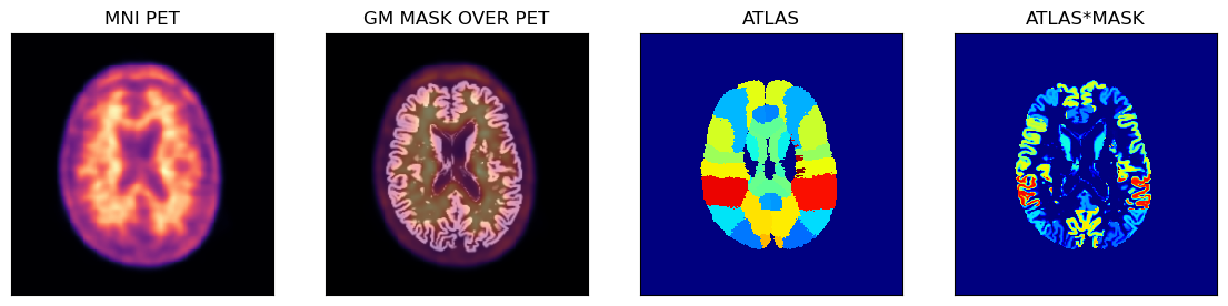
Upsampling PET to Higher Resolution Grid
The PET image can be upsampled to higher resolution grid without any extra modifications (apart from interpolation if chosen) in order to obtain higher sampling accuracy from the structural information provided by the T1w MRI images and their derivates (segmentations, etc.).
Upsampling With and Without Interpolation
Below is shown the Python code to trim and upscale the PET image to roughly the same voxel size as the MRI using nimpa.imtrimup command. The upscaling is governed by the scale parameter, which in this case is 2 to bring the voxel size from approximately 2 mm to 1 mm isotropically.
The interpolation is controlled by the int_order parameter, which is 1 meaning that trilinear interpolation is used. If int_order = 0, no actual interpolation is used resulting in True-Voxel or Native-Voxel upsampling in which the same voxel values are preserved by many more smaller voxels, thus avoiding any interpolation effects if desired so.
    # > upscale and trim the original PET and use linear interpolation (if no interpolation is desired then use int_order=0)
    imupd = nimpa.imtrimup(fpetin, scale=2, int_order=1, store_img=True)

    # > get the upscaled PET space atlas and probability GM/WM masks
    natupdct = amypet.atl2pet(hmr['fatlas_full'], out_cl, fpet=imupd['fim'], outpath=onat)
The upscaled images and sampling masks are shown below.
# > plot the images
fig,axs = plt.subplots(1,4, figsize=(14, 8))
axs[0].matshow(imupd['im'][80,...], cmap='magma')
axs[1].matshow(imupd['im'][80,...], cmap='magma')
axs[1].imshow(natupdct['gmpet'][80,...], cmap='gray', alpha=0.5)
axs[2].matshow(natupdct['atlpet'][80,...], cmap='jet')
axs[3].matshow(natupdct['atlpet'][80,...]*natupdct['gmpet'][80,...], cmap='jet')
# > remove ticks
for i in range(4):
    axs[i].axes.get_xaxis().set_ticks([])
    axs[i].axes.get_yaxis().set_ticks([])

axs[0].set_title('MNI PET')
axs[1].set_title('GM MASK OVER PET')
axs[2].set_title('ATLAS')
axs[3].set_title('ATLAS*MASK');