Atlas-Based MNI PET analysis
The analysis relies on the CL processing presented previously in the previous section Centiloid Pipeline.
The presented MNI space analysis of PET images may use either the MNI normalised PET images, or the output CL/UR images stored in the results subfolder in the output path stored in cl_out['opth'] - the output dictionary of the CL pipeline (see details here). For the MNI analysis a number of generally available atlases can be used as shown below.
Atlases Supported In AmyPET
The available atlases include:
- The Hammers atlas (you will be prompted to fill the online license).
- The DKT (Desikan-Killiany-Tourville) atlas.
- The Schaefer atlas.
- The AAL atlas.
# > get the available atlases in the MNI space as Python dicionaries
hmr = amypet.get_atlas(atlas='hammers')
dkt = amypet.get_atlas(atlas='dkt')
sch = amypet.get_atlas(atlas='schaefer')
aal = amypet.get_atlas(atlas='aal')
All the atlases come with the sub-dictionaries of available labels and names. For example, for the Hammers atlas, we can find the following dictionary items:
hmr.keys()
dict_keys(['fatlas', 'fatlas_full', 'flabels', 'voi_lobes', 'vois'])
with vois and voi_lobes representing the different labels for all the available volumes of interests (VOI) and the composite VOIs for the lobes of the brain. Please note that the Hammers atlas has the full version (including the white matter, WM) and the grey matter (GM) version.
Atlas resampling to the PET image size
Although the available atlases are already in the MNI space, they have a different image or voxel sizes. Hence they are interpolated with identity transformation to fully align them with the PET space which can have voxel size of either 1 or 2 mm isotropically.
# > Hammers atlas - the grey matter version
fhmr = spm12.resample_spm(
    out_cl['fnorm'][1],
    hmr['fatlas'],
    np.eye(4),
    intrp=0,
    fimout=Path(out_cl['fnorm'][1]).parent/('InPET_'+hmr['fatlas'].name),
    del_ref_uncmpr=True,
    del_flo_uncmpr=True,
    del_out_uncmpr=True)

# > Hammers atlas - full version with the WH
fhmrf = spm12.resample_spm(
    out_cl['fnorm'][1],
    hmr['fatlas_full'],
    np.eye(4),
    intrp=0,
    fimout=Path(out_cl['fnorm'][1]).parent/('InPET_'+hmr['fatlas_full'].name),
    del_ref_uncmpr=True,
    del_flo_uncmpr=True,
    del_out_uncmpr=True)

fdkt = spm12.resample_spm(
    out_cl['fnorm'][1],
    dkt['fatlas'],
    np.eye(4),
    intrp=0,
    fimout=Path(out_cl['fnorm'][1]).parent/('InPET_'+dkt['fatlas'].name),
    del_ref_uncmpr=True,
    del_flo_uncmpr=True,
    del_out_uncmpr=True)

fsch = spm12.resample_spm(
    out_cl['fnorm'][1],
    sch['fatlas'],
    np.eye(4),
    intrp=0,
    fimout=Path(out_cl['fnorm'][1]).parent/('InPET_'+sch['fatlas'].name),
    del_ref_uncmpr=True,
    del_flo_uncmpr=True,
    del_out_uncmpr=True)

faal = spm12.resample_spm(
    out_cl['fnorm'][1],
    aal['fatlas'],
    np.eye(4),
    intrp=0,
    fimout=Path(out_cl['fnorm'][1]).parent/('InPET_'+aal['fatlas'].name),
    del_ref_uncmpr=True,
    del_flo_uncmpr=True,
    del_out_uncmpr=True)
Exploring The Atlases
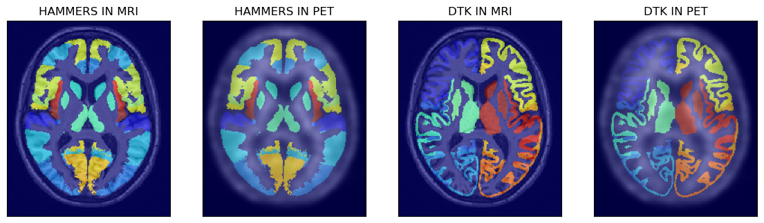
All the four available atlases are shown below after loading the atlases to Numpy arrays:
# > read the atlases to Numpy arrays
ihmr = nimpa.getnii(fhmr)
idtk = nimpa.getnii(fdkt)
isch = nimpa.getnii(fsch)
iaal = nimpa.getnii(faal)
# > show the first two atlases superimposed on MRI and PET images
fig,axs = plt.subplots(1,4, figsize=(14, 8))
axs[0].matshow(mrin[100,...], cmap='gray')
axs[0].imshow(ihmr[100,...], cmap='jet', alpha=0.6)
axs[1].matshow(petn[100,...], cmap='gray')
axs[1].imshow(ihmr[100,...], cmap='jet', alpha=0.5)
axs[2].matshow(mrin[100,...], cmap='gray')
axs[2].imshow(idtk[100,...], cmap='jet', alpha=0.6)
axs[3].matshow(petn[100,...], cmap='gray')
axs[3].imshow(idtk[100,...], cmap='jet', alpha=0.5)
# > remove ticks
for i in range(4):
axs[i].axes.get_xaxis().set_ticks([])
axs[i].axes.get_yaxis().set_ticks([])
# > image labels
axs[0].set_title('HAMMERS IN MRI')
axs[1].set_title('HAMMERS IN PET')
axs[2].set_title('DTK IN MRI')
axs[3].set_title('DTK IN PET')
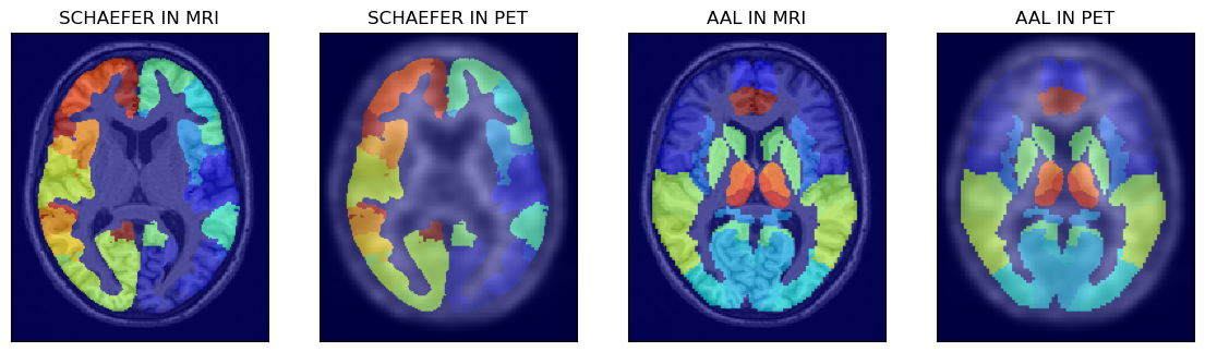
# > show the other two atlases superimposed on MRI and PET images
fig,axs = plt.subplots(1,4, figsize=(14, 8))
axs[0].matshow(mrin[100,...], cmap='gray')
axs[0].imshow(isch[100,...], cmap='jet', alpha=0.6)
axs[1].matshow(petn[100,...], cmap='gray')
axs[1].imshow(isch[100,...], cmap='jet', alpha=0.5)
axs[2].matshow(mrin[100,...], cmap='gray')
axs[2].imshow(iaal[100,...], cmap='jet', alpha=0.6)
axs[3].matshow(petn[100,...], cmap='gray')
axs[3].imshow(iaal[100,...], cmap='jet', alpha=0.5)
# > remove ticks
for i in range(4):
axs[i].axes.get_xaxis().set_ticks([])
axs[i].axes.get_yaxis().set_ticks([])
# > image labels
axs[0].set_title('SCHAEFER IN MRI')
axs[1].set_title('SCHAEFER IN PET')
axs[2].set_title('AAL IN MRI')
axs[3].set_title('AAL IN PET')
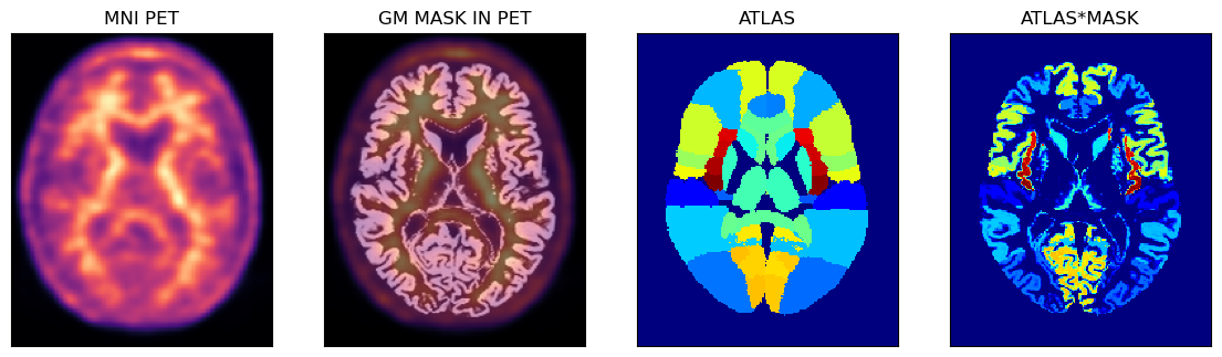
PET Image Analysis Using The Hammers Atlas And The GM Probability Mask
Below is an example of using the PET image in the MNI space with the corresponding GM probability mask (thus avoiding some partial volume problems during sampling) and the full Hammers atlas with segmentations for the GM and WM.
# > get the Numpy array representing the Hammers atlas image
ihmrf= nimpa.getnii(fhmrf)

# > the the Numpy array of the PET image in the MNI space
petmni = nimpa.getnii(out_cl['fnorm'][1])

# > get the corresponding GM probability mask Numpy array
gm_mni = nimpa.getnii(out_cl['fnorm'][2])

# > plot the images
fig,axs = plt.subplots(1,4, figsize=(14, 8))
axs[0].matshow(petmni[100,...], cmap='magma')
axs[1].matshow(petmni[100,...], cmap='magma')
axs[1].imshow(gm_mni[100,...], cmap='gray', alpha=0.5)
axs[2].matshow(ihmrf[100,...], cmap='jet')
axs[3].matshow(ihmrf[100,...]*gm_mni[100,...], cmap='jet')

# > remove ticks
for i in range(4):
    axs[i].axes.get_xaxis().set_ticks([])
    axs[i].axes.get_yaxis().set_ticks([])

axs[0].set_title('MNI PET')
axs[1].set_title('GM MASK IN PET')

axs[2].set_title('ATLAS')
axs[3].set_title('ATLAS*MASK');
Perform the extraction of average VOI values
For simplicity here we use the composite lobe VOIs:
vois = amypet.extract_vois(
    petmni,
    fhmrf, # uses full atals
    hmr['voi_lobes'],
    atlas_mask=gm_mni, # applies the GM mask on top of the full Hammers atals
    outpath=outpath/'MNI_masks', # path to the masks
    output_masks=True # output all the individual masks for each composite VOI
)
Average value for the cingulate gyrus
print('The average value in the cingulate gyrus is avg = {}. The number of voxles (also partial) is nvox = {}.'.format(vois['CG']['avg'], vois['CG']['vox_no']))
The average value in the cingulate gyrus is avg = 9066.670901759866. The number of voxels (also partial) is nvox = 26160.29958630912.